FE 'tkGooies'

'IMAGE animations'
group

A Tk GUI to
Animate Two
Sinusoidal Waves
Merging

waves from Two
Point-Sources
(or slits)

(FE = Freedom Environment)

FE 'tkGooie' interface for the
simulation of 2 sinusoidal
waves merging
---
with choice of 3
colors for the peaks,
neutral, and troughs
of the merged wave
---
and with animation
start and stop
radiobuttons

FE Home Page > FE Downloads Page >

FE 'tkGooies' Description Page >

FE 'tkGooies' 'IMAGEanimations' Page >

This
'Two-Waves-Merging Simulation/Animation'
tkGooie Page

INTRODUCTION to
Tcl-Tk Code for a GUI to
simulate and animate
Two Sinusoidal Waves Merging ---
waves from Two Point-Sources'

For about a year now (circa 2015), I have been planning to make a Tk GUI that performs an image animation of two waves interfering, like in the classic still images of two waves emanating from two 'slits' or 'point-sources' creating an 'interference pattern', like the following diagram by the scientist Thomas Young, circa 1800.

There are multiple reasons why I wanted to make this image animation, including:

  • I plan to make an 'Audio Visualizer' someday via a Tcl-Tk script.

    This planned visualizer is to be driven by audio input --- OR other types of varying input, such as activity from a network-interface card or by monitoring CPU-activity.

    Making a 'visualizer' for any of these types of activity would require generating some rather complex images at a rather fast 'frame-rate'.

    I could use this 'two-waves-merging' animation to determine what I might need to do to generate images at a sub-second rate.

  • I am a math, physics, and other sciences aficionado who likes to use Tcl-Tk to make math-physics-science topics easier to visualize and explore.

    This 'app' is an 'arrow' that I would like to add to that 'quiver' of tools.

  • The usual depictions of two waves interfering make a lot of simplifying 'assumptions' --- such as both waves having the same frequency, the source of both waves being 'in phase', both waves having the same max-amplitude.

    Furthermore, the colors in most stills and animations are fixed, with no option for me to make a change in the colors used.

    I wanted to make a utility that allows for differing frequencies, phases, amplitudes, wave-velocity, and colors.

    I also wanted to allow for adjusting the distance between the 2 point sources.

  • Even if this 'app' does not have much scientific value, I may find use for it as a decorative-image-generator.

    Since this animation is rather 'pseudo-scientific', I plan to implement this 'app' in an 'IMAGEanimations' sub-menu of the 'IMAGEtools' menu of the FE 'tkGooies' system --- rather than in a 'MATHtools' menu or some 'science-tools' menu.

    That is, this 'app' might have more use as a maker of decorative image backgrounds, rather than as an elucidator of physical principles.

    However, this 'app' depends on a fair amount of mathematical manipulation, which makes it (or its code) a candidate for inclusion in the 'MATHed' (math education) sub-menu of the 'MATHtools' menu of the 'tkGooies' system.

    (A 'Help' button on the GUI can be used to explain the math and code involved.)

These were more than enough reasons to motivate me to get started in coding this Tk script.


Basic Goals of the Tk Script:

My purpose for this Tk GUI script is/was to generate an animation of 2 circular wave patterns interfering (merging).

The animation is to be shown in a rectangular Tk 'photo' image on a rectangular Tk 'canvas' widget.

The resultant wave amplitude at any point in the image is to be the algebraic sum of the two amplitudes of the 2 waves at the point.

The resultant amplitude at any point in the rectangular image area is to be plotted as a pixel color.


Method of Math Modelling of the Amplitudes:

The typical mathematical representation of a sinusoidal wave-form as a function of both time and space is typically given by

in which

  • 'A' is an AMPLITUDE
  • 'f' is a FREQUENCY
  • 'v' is a WAVE-VELOCITY
  • lambda is WAVELENGTH, which = v / f
  • 'x' is a distance

Alternatively, the math representation can take slightly different forms, such as

I decided to take the following approach --- specific to the rectangular image area on the GUI.

The two waves are modelled as coming from two 'sources' or 'slits' at the bottom of the rectangular image.

The pixels of the image area (in integer coordintes --- i,j) are mapped to 'real', 'floating-point' 'world coordinates' --- (x,y).

We imagine the two waves traveling at a common velocity

v = f * L

where 'f' is frequency (say, cycles per second) and 'L' is wave length (say, inches or centimeters or meters or whatever per cycle).

So f = v / L   and   L = v / f.

Actually, we will allow our two merging waves to have their own frequency and wave length --- f(i) and L(i) where i = 1 and 2.

But we think of velocity v being the same for both waves, since we are simulating 2 waves traveling in the same medium (water, vacuum, air, granite, glass, whatever).

The amplitude of wave 'i', where i = 1 or 2, is given by a sinusoidal equation representing the amplitude of a 'traveling wave'


   A(i,x,y,t) = A(i) * sin ( (2 * pi * f(i) * t) - ( 2 * pi* r(i,x,y) / L(i) ) + ph(i) )

                       term-1 (time-dependent)     term-2 (distance-dependent)   term-3 (phase)


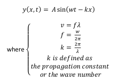
where there are 3 terms in the sin function and where A(i) and ph(i) are constants for wave i --- 'A' being an amplitude factor and 'ph' being a phase angle.

    (We allow for two different 'initial' phase angles for the 2 waves. In other words, we allow for simulating 2 waves that are NOT in sync at their sources, even when their two frequencies are equal.)

f(i) and L(i) are the frequency and wave-length of wave i.

The term ( 2 * pi * f(i) * t ) represents the sinusoidal variation with time, t, of the wave amplitude at any point (x,y) --- converted to radians.

The term ( 2 * pi * r(i,x,y) / L(i) ) represents the number of wave-lengths from the source-point to the point (x,y) --- converted to radians.

r(i,x,y) represents the distance from the source-point of wave i.

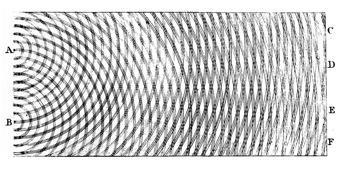
Let us say (x1,y1) and (x2,y2) are the 2 source points. Then

r(1,x,y) = sqrt( (x-x1)^2 + (y-y1)^2 )

and

r(2,x,y) = sqrt( (x-x2)^2 + (y-y2)^2 )

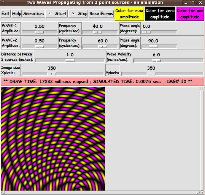
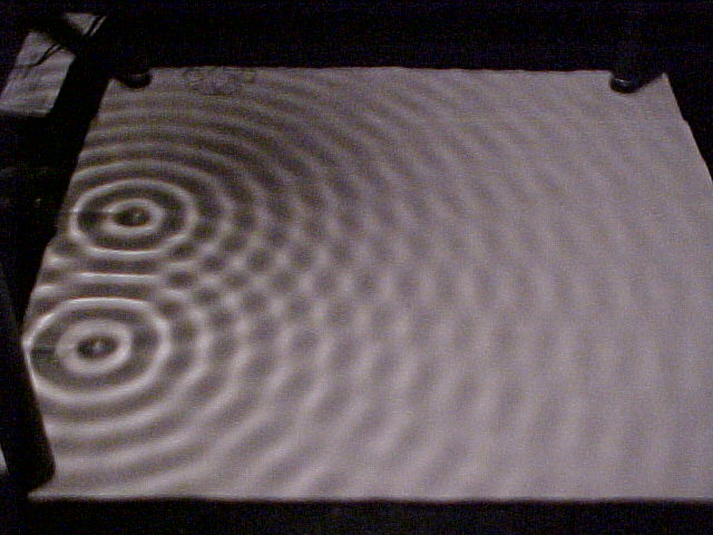
We will let the 2 source points be on the bottom of the image rectangle at y=0.

We will let the origin (0,0) be in the middle of the bottom of the rectangle.

We let the two source points be a distance 'd' on either side of the origin.

The resultant amplitude (RA) of the 2 merged waves at time t and at point (x,y) is given by

A(1,x,y,t) + A(2,x,y,t).

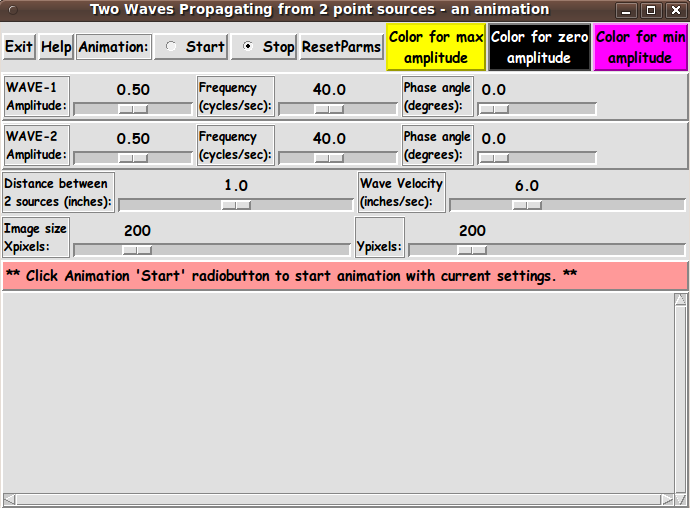
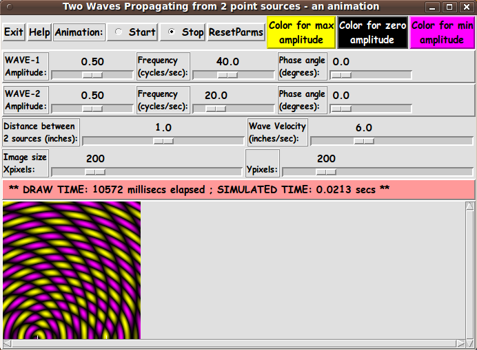
The Tk GUI allows the user to specify positive constants for the numbers f(i), L(i), A(i), ph(i), and 2d (the distance between the two point sources).

    (Actually, we let the user specify wave-velocity, v, rather than L(1) and L(2).

    We calculate L(i) = v / f(i).)


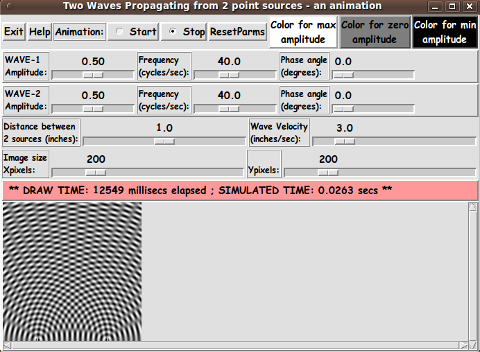
Method of Math Conversion of
the Resultant-Amplitude to Color:

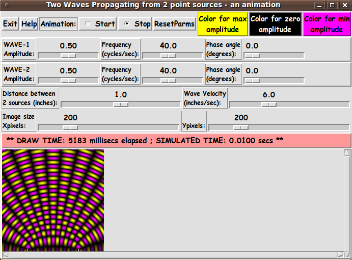
The amplitude of the waves are depicted with colors interpolated between a 'max-color' and a 'min-color'.

In fact, we allow for specifying a 3rd 'zero-color'.

For positive amplitudes, we interpolate between 'max-color' and 'zero-color'.

For negative amplitudes, we interpolate between 'min-color' and 'zero-color'.

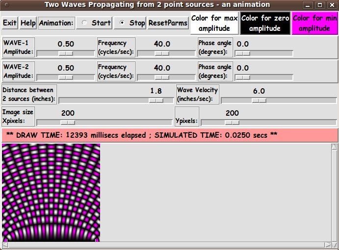
So the Tk GUI is to have 3 buttons by which to specify the

  1. max-color
  2. zero-color
  3. min-color

We use the sum of the 2 max-amplitudes

Asum = A(1) + A(2)

to do the interpolation.

When resultant amplitude

RA = A(1,x,y,t) + A(2,x,y,t)

is positive, we get the color for RA from


   RA-color = (RA/Asum) * max-color + (1 - RA/Asum) * zero-color

         where RA/Asum and (1 - RA/Asum) are between 0 and 1


and when RA is negative, we get the color for RA from


   RA-color = (abs(RA)/Asum) * min-color + (1 - abs(RA)/Asum) * zero-color

         where abs(RA)/Asum and (1 - abs(RA)/Asum) are between 0 and 1


    Actually, we use 3 interpolations to get RGB colors for RA.
    For example:

    Let r = abs(RA) / Asum .

    RA-R = ( r * max/min-color-R ) + ( (1 - r) * zero-color-R )
    RA-G = ( r * max/min-color-G ) + ( (1 - r) * zero-color-G )
    RA-B = ( r * max/min-color-B ) + ( (1 - r) * zero-color-B )

    We use max or min color depending on whether RA is positive or negative.

    The RGB values for max-color, zero-color and min-color are integers between 0 and 255.

    The 3 RGB values for RA are also kept between 0 and 255.


Method of Putting the Pixel Colors on
Each of the animation Images:

This script makes a sequence of color-shaded images by making a sequence of images in a Tk 'photo' image 'structure' that is placed on a Tk canvas widget.

The in-memory image 'structure' is created by an 'image create photo' command.

The image 'structure' is put on the Tk canvas via a Tk canvas 'create image' command --- and each image in the animation sequence is generated via

put <hexcolor> -to $i $j

commands on the image.

Actually, to reduce the number of 'put' commands, we build each entire image as a list-of-lists-of-hexcolors and use one 'put' to put the list-of-lists in the image structure on the canvas.


Assembling the pieces   (The GUI)

Now it was a matter of putting the pieces together.

I took 'code-pieces' from some of my other Tk scripts that make color-shaded, 3D-like images on a Tk canvas.

I ended up with the following GUI as an initial display.

If you take the hint in the message line of the initial GUI and simply click on the 'Start' radiobutton, the default settings are used and animation images like the following are generated.

You can see two very small, thin (one-pixel wide) white lines at the bottom of the GUI.

Those two lines indicate the location of the 2 simulated 'point-sources' of the 2 waves.

You can use the 'Distance' scale widget on the GUI to move those two points wider apart or closer together.

Colors

Note that I have supplied 3 buttons on the GUI with which to set the 'max-amplitude' color, the 'zero-amplitude' color, and the 'min-amplitude' color.

Those 3 buttons call on an 'external' color-selector-GUI script to set those colors.

You can make that color-selector script by cutting-and-pasting the code from the page that offers a non-obfuscated color selector GUI on this site.

    To get colors like you see in various 'classical' gray-scale still and animated images, you may find that you may want to use 'white', 'gray', and 'black' for the 'max', 'zero', and 'min' colors.

    Those colors yield animation images like the following.

Below is an example where the initial yellow for 'max-amplitude' is changed to white --- and where the two sources were simulated to be farther apart.

In this simulation GUI, the bottom left and right corners of the image are always simulated to be at (-1,0) and (+1,0) --- in 'world-coordinates'. Hence the 'Distance' scale widget allows you to set the distance between the 2 point-sources to be a maximum of 2.0 units apart.

    The distance to the top of the image, in 'world-coordinates', is always determined according to the aspect-ratio that the user determines for the image --- by setting the Y-pixels scale widget.

    For a square image, the top left and right corners of the image area are considered to be at world-coordinate-points (-1.0,+2.0) and (+1.0,+2.0).

Frequencies

Below is an example where the two frequencies are different --- 40.0 and 20.0.

This indicates how you can get 'swirly' patterns --- and an appearance like twisted threads of colored yarn.

Although the labels in the 'Distance' and 'Velocity' labels for those two scales say 'inches', you can imagine the distance units being whatever you want --- centimeters or feet or yards or meters or micrometers or nano-meters or whatever.

I put 'inches' to help me think in terms of a wave moving across the 20-inches or so of my computer monitor.

Phases and Amplitudes

I did a couple of experiments where I simply changed a phase of one of the waves (to 90 degrees and 180 degrees).

The animations did not look much different from the 'initial display' image above.

It just appeared that the 'lumps of color' move over a little bit.

Also, I did an experiment where I simply changed an amplitude of one of the waves (from 0.5 to 1.0).

The animation did not look much different from the 'initial display' image above.

It just appeared that some of the 'lumps of color' were a little more faded (less intense).

Performance
(image generation time)

After generating the images above, I decided that this utility needed a display of the image-number of the animation --- as seen in the message line in the following image.

Note that for this animation, I changed the image-area from 200 x 200 pixels to 350 x 350 pixels. (I also used 2 different frequencies and changed one of the phase angles.)

The 'elapsed time' of the animation is shown on the message line.

    (I should have labelled that 'ANIMATE TIME' instead of 'DRAW TIME' ; corrected in the code below).

Also shown is the simulated 'physical' time --- and the number-of-images that have been generated in the animation.

Note that it took about 17 seconds to generate 10 images --- about 1.7 seconds per 350 x 350 pixels image.

The initial image size of 200 x 200 pixels took about 0.6 seconds per image.

For a smooth animation, we need about 20 images per second --- about 0.05 secs per image ; about 10 times faster (for 200x200 images).

And we need about 30 times faster for 350x350 images.

So, on my medium-powered desktop computer, the image generation was not fast enough for smooth animation, even when using the rather small 200x200 image size and even though I took steps to generate each image fairly efficiently.

When I developed the script that I posted at wiki.tcl.tk and on this site, at GUI for Drawing 'Super-ellipses', with nice shaded edges, I learned my lesson about needing to use braces with 'expr' statements --- for much better execution times.

    (Brent Welch et. al. point this out before page 8 in the 4th edition of 'Practical Programming in Tcl and Tk' --- although they do not follow this advice in many 'expr' examples later in the book.)

It made a huge difference, so, in this script (and in all my Tk scripts henceforth), I consistently use braces with ALL 'expr' commands --- in particular, in the compute-intensive 'animate' proc of this Tk script and in the procs that are called by 'animate'.

However, even though I took those precautions, it looks like it will take on the order of 0.25 to 0.5 seconds to draw each image --- even using a small image area and a top-end CPU of this era (circa 2016) --- and even after making further code-efficiency improvements.

    Perhaps if someone runs this code on a very high-end Intel 'i7' processor (of this 2016 era), they can observe some almost-smooth animations.

    As I noted above, on my desktop computer it was taking about 1.7 seconds to generate each 350 x 350 pixels image.

    My computer is an 'AMD Athlon X4 630' processor with 4 cores, but it may be using only one core to do most of the math in computing each pixel color.

    At the 'single-thread' CPU benchmarks page cpubenchmark.net/singleThread.html, my CPU has a 'Passmark' rating of 958, while various Intel 'i7' processors at the top of that page (in 2016 Mar) had Passmark ratings in the 2,000 to 2,500 range --- about 2 to 2.5 times higher than my CPU.

    Examples:

    • Intel Core i7-4790K - 2,530
    • Intel Core i7-6700K - 2,327
    • Intel Core i7-4770K - 2,260

    It is quite likely that one of these 'high-end' 'i7' processors would generate 350 x 350 images in about 0.8 seconds --- still about 16 times slower than the 0.05 seconds per image that would give a smooth animation.

    Even if 4 cores are doing the processing, we may not see the smooth animation we would like.

    The bottom line is that doing all these computations to determine the pixel colors of 350 x 350 = 122,500 pixels in each image is probably not going to give a smooth animation with the CPU's available in 2016 (and with a Tcl-Tk script).

Someday, I may add widgets to the GUI to support generating an animated-GIF file (or movie file) from a sequence of generated images.

With the animated-GIF or movie file, it will be possible to get a fairly smooth playback of the simulated merging of the two waves.


DESCRIPTION OF THE CODE

Below, I provide the Tk script code for this 'two-waves-merging' 'app'.

I follow my usual 'canonical' structure for Tk code, for this Tk script:


  0) Set general window & widget parms (win-name, win-position,
     win-color-scheme, fonts, widget-geometry-parms, win-size-control).

  1a) Define ALL frames (and sub-frames, if any).
  1b) Pack   ALL frames and sub-frames.

  2) Define & pack all widgets in the frames, frame by frame.
              Within each frame, define ALL the widgets.
              Then pack the widgets.

  3) Define keyboard and mouse/touchpad/touch-sensitive-screen action
     BINDINGS, if needed.

  4) Define PROCS, if needed.

  5) Additional GUI initialization (typically with one or more of
     the procs), if needed.


This Tk coding structure is discussed in more detail on the page A Canonical Structure for Tk Code --- and variations.

This Tk coding structure makes it easy for me to find code sections --- while generating and testing this script, and when looking for code snippets to include in other scripts (code re-use).


Experimenting with the GUI

As in all my scripts that use the 'pack' geometry manager (which is all of my 100-plus Tk scripts, so far), I provide the four main 'pack' parameters --- '-side', '-anchor', '-fill', and '-expand' --- on all the 'pack' commands for the frames and widgets.

I think I have found a good setting of the '-side', '-anchor', '-fill', and '-expand' parameters on the 'pack' commands for the various widgets of this GUI.

In particular ...

The 'canvas' widget expands/contracts appropriately when the window size is changed --- and button and label widgets stay fixed in size and relative-location as the window size is changed.

If anyone wants to change the way the GUI configures itself as the main window size is changed, they can experiment with the '-side', '-anchor', '-fill', and '-expand' parameters on the 'pack' commands for the various widgets --- to get the widget behavior that they want.

---

Additional GUI experimentation:
You could change the fonts used for the various GUI widgets. For example, you could change '-weight' from 'bold' to 'normal' --- or '-slant' from 'roman' to 'italic'. Or change font families.

In fact, you may NEED to change the font families, because the families I used may not be available on your computer --- and the default font that the 'wish' interpreter chooses may not be very pleasing.

Furthermore, there are variables used to set geometry parameters of widgets --- parameters such as border-widths and padding.

And you could change the '-relief' values for frames and widgets. Feel free to experiment with those 'appearance' parameters as well.


Some features of the code

There are plenty of comments in the code to describe what most of the code-sections are doing.

The most complex code is in the 'animate' proc.

See the comments in that proc to see how it is implemented.

See the top of the 'PROCS' section for a list of the procs used in this Tk script.

See comments in the procs for details on the purpose of each proc and for details on the methods by which each proc was implemented.

Here is a quick overview of the procs --- to give an idea of the 'guts' of this utility:


  - animate                   - called by a button1-release binding
                                on the 'Start' radiobutton.

  - setMappingVars_for_px2wc  - called by proc 'animate'

  - Xpx2wc                    - called by proc 'animate'
  - Ypx2wc                    - called by proc 'animate'

  - set_scale_Ymax_equal_Xmax - called by button1-release binding on the
                                X-imgsize scale widget

  - set_max_color1            - called by color1 (max) button '-command'

  - set_min_color2            - called by color2 (min) button '-command'

  - set_zero_color0           - called by color0 (zero) button '-command'

  - update_color_button       - called by the 'set_*_color*' procs and once
                                in the 'Additional GUI Initialization section.

  - reset_parms               - called by 'Reset' button and in the
                                'Additional GUI Initialization' section,
                                to initialize the parms.

  - advise_user               - called by the 'animate' proc and various bindings
 
  - popup_msgVarWithScroll    - called by 'Help' button


One thing that I discovered in testing a previously-created GUI is a 'trick' to make the GUI (in particular the 'canvas' area) resize nicely after a change to the image-size via the x and y image-size scale widgets.

It turned out that the resizing would not occur after the tester (me) would resize the window by tugging on an edge or corner of the window. The resizing would occur nicely before that 'manual intervention' with the window manager.

It turned out that a Tk 'wm' (window manager) command --- namely

wm geometry . {}

can be used to restore the nice auto-resizing of the canvas area around the image area.

By some searches on wiki.tcl.tk (with terms like 'wm resize'), I found this 'trick' used on the page http://wiki.tcl.tk/10720 (weeEdit) --- in the '-command' of a 'Resize window' button.

In that code, the 'wm geometry . {}' statment was being used to resize a 'text' widget, not a 'canvas' widget.

A search on 'wm geometry . {}' at wiki.tcltk revealed that this 'wm statement' was mentioned in a section titled 'word Wrap Via Tk Text Widget' --- on the page http://wiki.tcl.tk/44 (Additional string functions) --- with the comment 'Make sure the toplevel shrinks or expands to fit'.

Thanks to 'D.McC' (David McClamrock) for revealing this technique to me.

I have never seen this 'toplevel shrink/expand' technique --- using 'wm geometry . {}' --- mentioned in the Tcl-Tk books that I have used the most --- the Eric Foster-Johnson books and the Brent Welch books.

But I did find mention of this capability in the original 1994 edition of the John Ousterhout Tcl-Tk book --- on page 237 --- where it says:

    "If you would like to restore a window to its natural size, you can invoke 'wm geometry' with an empty geometry string:

    wm geometry . {}

    "This causes Tk to forget any size specified by the user or by 'wm geometry' so the window returns to its natural size."

Apparently 'wm geometry . {}' can be used to cause Tk to signal the window manager to resize the toplevel window according to the widget sizes within the window --- for example, after a user has 'manually' resized the toplevel window by 'tugging' on a window edge or corner.


Comments in the Code

It is my hope that the copious comments in the code might help Tcl-Tk coding 'newbies' get started in making GUI's like this.

Without the comments --- especially in the 'animate' proc --- the code might look even more cryptic than it already is.

Without the comments, potential young Tcler's might be tempted to return to their iPhones and iPads and iPods --- to watch videos of large meteors streaking across the sky and busting out windows for miles around --- and, luckily/hopefully, not impacting near a nuclear reactor. (Near a few wind turbines --- not NEARLY so bad.)


The Tcl-Tk Script CODE

Here is a link to CODE for the Tk script
'twoSinusoidalWavesMerging_twoPointSources.tk'.

With your web browser, you can 'right-click' on this link --- and in the menu that pops up, select an item like 'Save Link Target As ...' --- to save this file to your local computer.

Then you can rename the file to remove the '.txt' suffix. Make sure that you have execute permission set on the file --- in order to execute the script.

Some Physical Considerations
(correlation with 'the real world')

In doing some web searches related to writing this 'app', I ran across the Wikipedia page on Dispersion of water waves.

That page indicated that the math expressions for modelling water waves can seem to be quite challenging to understand --- especially when you start considering phenomena like group-velocity and phase-velocity of interacting water waves, as the following animation indicated.

And a sloping sea floor can introduce further complications into the wave forms in the case of waves in shallow areas.

However, I was encouraged that the simulation with this 'app' might correlate fairly well with 'real world' wave action, when I saw aerial photos like the following.


This photo indicates that planar waves impinging on a small opening
do indeed generate circular waves that behave in a way that we can
represent with our sinusoidal math expression.


This photo indicates that gaps in a barrier to waves do indeed
generate circular waves from the gaps -- waves that spread and 'interfere'
in the manner that we can represent with our 2 sinusoidal math expressions.

Besides these aerial photos, the results from 'ripple tank' experiments also indicate that our 2 sinusoidal math expressions give a pretty good computer-simulation of what happens in a tank of water. Here is a diagram of a ripple tank --- including a motor and bar that can be used to generate 'straight waves'.

Here is a diagram that shows how the motorized bar could be equipped with a 'rod dipper' to generate 'circular waves' --- instead of 'straight waves'.

Here is a diagram that shows how a barrier could be introduced in the ripple tank to generate a circular wave from a 'straight wave'.

Here is a photo that shows how 2 rod dippers could be used to generate 2 circular waves --- to study their interference patterns.

Here is an image that shows the results from such a '2-rod-dipper' experiment.

It looks quite similar to the gray-scale simulation that was shown above.

Diagrams like the following remind one that there are multiple types of wave phenomena that could be simulated.

This 'app' is emulating 'diffraction' --- not 'reflection' or 'refraction' or 'absorption'.

Diagrams like the following two remind one that this 'app' is treating the special case of modeling diffraction of waves from a very small opening --- not wide openings.


If the opening is wider and we were attempting to model planar waves impinging
on the opening, then circular wave propagation would not properly
emulate/approximate what happens in 'the real world'.


The flat barrier at the bottom right indicates that circular
diffraction patterns are generated from the ends of such barriers.
The 'app' presented on this page does not attempt to emulate the
types of wave generation seen in the bottom two parts of this diagram.

Some possible FUTURE ENHANCEMENTS

There are quite a few enhancements that could be considered for this script, such as:

  • 1) Write-Ani-GIF:

    As I mentioned above, it may be good to offer an option to write an animated-GIF file from the sequence of images in this animation.

    It would certainly be more convenient than having to do a bunch of image captures and manually contruct an animated-GIF (or movie) file from the sequence of images.

    I have implemented a Write-Ani-GIF option in several 'tkGooies' in the 'IMAGEtools' group, such as:

    I can use code from one or more of those Tk scripts to make it relatively easy to implement a Write-Ani-GIF option.

  • 2) Radius-Dependent-Amplitude:

    I kind of glossed over the fact that in the math expressions for the two waves, I used a constant for the amplitude factor for the two waves.

    In actuality, the energy concentrated at the point source gets dissipated as the energy (wave front) proceeds away from each point source.

    If we imagine that the wave is confined to a 2D-rather-than-3D expansion, we can expect the two amplitudes to 'fall off' as the reciprocal of the radii in the two math expressions.

    And if we imagine that the wave is expanding in 3D (and we imagine that we are looking at a 2D cross-section of the wave-expansion in 3-space), we can expect the two amplitudes to 'fall off' as the reciprocal of the SQUARE of the two radii (like the influence of gravity of a planet falls off as the reciprocal of the square of the distance from the center of the planet).

    So to perform a more realistic simulation of water-waves expanding on the surface of a body of water, for example, we could use 'a-constant-A-over-r' rather than 'a-constant-A' as the amplitude factor in the two math expressions for the 2 waves.

      (To avoid a singularity at r=0, we could use 'a-constant-A-over-one-plus-r'.

      This would give amplitude A at r=0 and a 'one-over-r' fall-off of amplitude as r gets large.)

    Furthermore, to get a realistic simulation of electro-magnetic radiation or sound-radiation in 3D space, we could use 'a-constant-A-over-r-squared' rather than 'a-constant-A' as the amplitude factor in the two math expressions for the 2 waves.

      (To avoid a singularity at r=0, we could use 'a-constant-A-over-one-plus-r-squared'.

      This would give amplitude A at r=0 and a 'one-over-r-squared' fall-off of amplitude as r gets large.)

    To implement these 2D and 3D amplitude factors (as well as the current constant-amplitude formulation), we could add 3 radiobuttons to the GUI to allow the user to choose among 3 different amplitude-factor formulations --- constant, one-over-r, and one-over-r-squared.

      I postpone an in-depth discussion of avoiding the singularity at r=0 to a later time --- such as when I ever get around to implementing these amplitude radiobuttons.

  • 3) Another image area (narrow) to show an
    interference pattern on the 'top wall':

    I could add a Tk canvas image area, at the top of the main image, on which to draw an image representing the 'interference pattern' of the waves if we imagine them meeting on a wall at the top of the main image area.

    We could make this image area about 20 pixels high and as wide as the image in the main image area.

    We could easily draw this image by using 'create line' commands on a Tk canvas, and draw each (vertical) line in the same color as the colors of the pixels on the top line of pixels of the main image area.

    This image would then look like the 'intererence pattern on a wall' that is often seen in physics textbooks when they discuss the results of a 'double-slit' experiment.

  • 4) Another narrow image area to show
    a 'moving graph' of the resultant amplitude
    at a particular point in the main image area:

    I could add a Tk canvas image area, say at the bottom of the main image, on which draw points (for each time step) representing the 'amplitude height' at a particular point in the main image area.

    We could make this image area about 100 pixels high and about as wide as the image in the main image area.

    We could easily draw this image by using 'create point' commands on a Tk canvas, and draw each point at a height (positive or negative) corresponding to the resultant amplitude at the point (and at a current time step).

    This graph of 'resultant amplitude' (a combination of two sinusoidal functions) could be a 'marching-history' graph that depicts a recent history of the ampltude at the particular point.

    It would be similar to the animated GIF toward the top of this page (just above the aerial photos) that shows a moving-curve graph.

    We could choose a fixed point at which we 'sample' the amplitudes --- OR we could allow the user to pick a point on the main image area (and denote that point with a 'create oval' command on this lower Tk canvas).

  • 5) Change Scale Limits:
    (velocity and 2 frequencies)

    I chose the scale limits for the 2 frequency scale widgets and the velocity scale widget rather arbitrarily (but I was thinking of speed and frequencies of waves traveling across the surface of the computer monitor --- about 12 inches across).

    As an alternative (which will junk-up the GUI with perhaps too many widgets), we could add some radiobuttons (and other widgets) to the GUI by which the user can choose to emulate water-surface-waves, sound-waves, or electro-magnetic waves.

    One problem with this is that, in the case of electromagnetic (EM) waves, the frequencies can range over a huge range --- from 10-to-the-zero to 10-to-the-24 or more.

    And the wave-velocity can vary somewhat, depending on whether we are emulating EM waves through vacuum, air, water, glass, or whatever.

    The following two horizontal and vertical representations of the EM-spectrum indicate the range over which the frequencies (and wave-lengths) can vary.

    And with emulating sound waves, the speed of sound through various media can vary over a range of about 10-to-the-zero to 10-to-the-4 (meters-per-second) --- a rather wide range to be handled by a 'scale' widget by itself.

    So picking a way of making the choice of the 2 frequencies and the velocity quite meaningful to the user --- for a wide variety of physical wave phenomena --- can be quite a challenge in the design of the GUI.

    If I am just going to use this Tk script to generate some interesting/decorative individual images, then I am not going to be motivated to spend a lot of time on coming up with a user-friendly design to handle 'the units' in simulating water, sound, and EM waves over almost their entire possible physical range of frequencies, wave-lengths, and velocities.

  • 6) More efficiency of math operations:

    I indicated above that it would be nice to make the generation of the individual images at least 10 times faster --- especially if one wants to generate large images similar to HDTV resolution of 1920 x 1080 pixels.

    But, again, if I am just going to use this Tk script to generate some interesting/decorative images, then I am not going to be motivated to spend a lot of time on trying to achieve significant speed-up --- especially when a speed-up of 'an order of magnitude' is probably not going to be possible when limited by the speed with which the 'wish' interpreter can perform the math calculations within the 'expr' statements --- even if those arithmetic statements could be optimized to the max.

---

Of the several possible enhancements listed above, items 1, 2, 3, and 4 seem to be the most likely to be worth pursuing --- to do a better job of examining the wave interference phenomena.

But I should point out that others have gotten pretty ambitious. Some people have written apps to emulate wave patterns in the presence of other types of sources and barriers and reflectors.

---

In doing some web searches on terms like 'ripple tank', I found that someone has written a 'ripple tank applet' --- as seen in the following GUI.

Here they are emulating THREE point-sources --- from a 'triple slit'.

Note that they chose 'Setup Triple Slit'.

It appears that this app is meant to allow the user to add barriers (walls) of various kinds to the 'virtual ripple tank' --- as seen in the image below --- via 'Setup Half Plane'.

The following 2 images indicate that ripple tank experiments show that the emulation above is realistic.

The bottom line here is that there is a plethora of possible enhancements that could be made to a Tk GUI 'app' like this.

One advantage of this Tk script is that it is 'open' code --- available to anyone for enhancement. (And, as a bonus, it generates quite nice quality images.)


IN CONCLUSION

As I have said on several other code-donation pages on this freedomenv.com site and on the Tclers' wiki at wiki.tcl.tk ...

There's a lot to like about a utility that is 'free freedom' --- that is, no-cost and open-source so that you can modify/enhance/fix it without having to wait for someone else to do it for you (which may be never).

A BIG THANK YOU to Ousterhout for starting Tcl-Tk, and a BIG THANK YOU to the Tcl-Tk developers and maintainers who have kept the simply MAH-velous 'wish' interpreter going.

Bottom of this page with
Tcl-Tk Code for a GUI to simulate
Two Sinusoidal Waves Merging
--- waves from Two Point Sources

--- a utility in the FE 'tkGooies' system,
in the 'IMAGEanimations' group.

To return to a previously visited web page location, click on the Back button of your web browser a sufficient number of times. OR, use the History-list option of your web browser.
OR ...

< Go to Top of Page, above. >

Page history:

This FE web page was created 2016 Feb 07.

This FE web page was changed 2016 Mar 01.
(Added a couple of possible enhancements --- and CPU speed info.)

Page was changed 2019 Mar 01.
(Added css and javascript to try to handle text-size for smartphones, esp. in portrait orientation.)

Page was changed 2019 Jun 15.
(Specified image widths in percents to size the images according to width of the browser window.)


NOTE:
This code may someday be posted in a page on the Tcler's Wiki --- wiki.tcl-lang.org --- formerly wiki.tcl.tk. If I do that, I may put a link to the page here.


Who is right-er? --- Young or Newton?
Light is wave or particle?